Concept of Box Plot (Tableau)

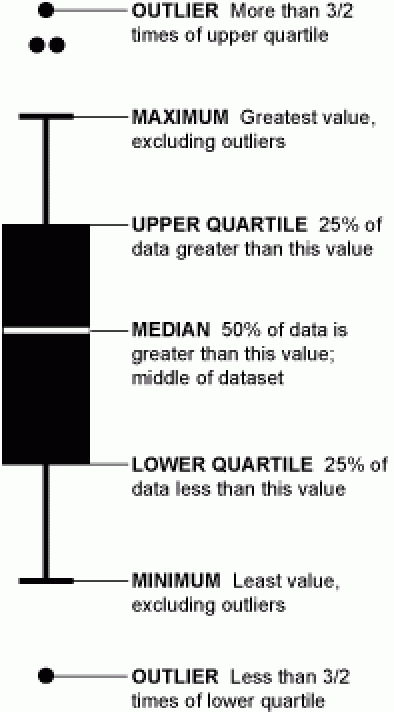
Box -plot is one of the prominent feature important for TABLEAU Statistics section of Examination. Below is simple example to clarify the concept for the individuals new to it.

A small example should make things clear. Consider a small village with 25 inhabitants. This is what they earn and the resulting box plot:

Citizen Nr.	Income	Key Value
25	3,001.25	Maximum
24	2,996.45
23	2,919.35
22	2,787.02
21	2,784.72
20	2,696.83
19	2,412.51	Q3: 0.75 * 25 = 18.75 = 19.
18	2,400.43
17	2,367.84
16	2,333.37
15	2,285.53
14	2,214.87
13	2,069.79	Median: 0.5 * 25 = 12.5 = 13.
12	1,923.62
11	1,819.22
10	1,773.34
9	1,597.54
8	1,589.48
7	1,494.65	Q1: 0.25 * 25 = 6.25 = 7.
6	1,423.74
5	1,391.92
4	1,334.88
3	1,184.53
2	1,125.78
1	1,005.85	Minimum

As you can see, the basic idea is to sort the data and then select the minimum, the maximum and the values at the referring positions: median (0.5), lower (Q1) (0.25) and upper quartile (Q3) (0.75). Why these values are considered to be robust statistic key values? In order to explain this, consider a similar village with one rich person and the following incomes:

Citizen Nr.	Income	Key Value
24	10,345.67	Maximum
23	2,919.35	Upper Bound
22	2,787.02
21	2,784.72
20	2,696.83
19	2,412.51
18	2,400.43	Q3: (18. + 19.)/2 = 2,406.47
17	2,367.84
16	2,333.37
15	2,285.53
14	2,214.87
13	2,069.79
12	1,923.62	Median: (12. + 13.) / 2 = 1,996.71
11	1,819.22
10	1,773.34
9	1,597.54
8	1,589.48
7	1,494.65
6	1,423.74	Q1: (6. + 7.) / 2 = 1,459.2
5	1,391.92
4	1,334.88
3	1,184.53
2	1,125.78
1	1,005.85	Minimum / Lower Bound

Changing Views Using Parameters

Create the parameters and calculated fields

Sample Worksheet -->https://public.tableau.com/profile/ritesh.bisht#!/vizhome/AdvanceParameterChangingViews/Select_Views_Fields

These steps use the Superstore sample to create a new parameter while you build the calculated field that will take advantage of it.

Step 1

Select Analysis > Create Calculated Field.

Step 2

In the Calculated Field dialog box, for Name, type Column 1 Category.

Step 3

Next to Parameters, click Create, and in the Create Parameter dialog box, complete the following steps.

1. Name the parameter appropriately so that viewers can tell what changing it will do. This example uses Select Column 1 Heading.
2. For Data type, select String.
3. For Allowable Values, select List, type None as the first value in the list, and then press Enter.
4. Complete the list by typing the names of the additional dimension fields that you want to expose through the parameter.Note: This example uses the customer name, customer segment, region, department, and category fields. These are all dimensions of the same data type (string). If you wanted to include a measure such as profit in this list, one option would be to convert the measure to a string value. You would do this when you build the calculated field, using the STR() function. This article covers only the single data type scenario.
5. The Display As aliases default to the field name, and for this exercise you can leave them as they are.
6. Click OK to return to the Calculated Field dialog box.

Step 4

Repeat the previous step to create the following additional parameters:

• Select Column 2 Heading
• Select Row 1 Heading
• Select Row 2 Heading

Tip: Instead of typing each value in the list, click Add from Parameter to add them from Select Column 1 Heading.

Step 5

In the Calculated Field dialog box, for Formula, build the following calculation:

CASE Select Column 1 Heading

WHEN 'Customer Name' THEN Customer Name

WHEN 'Customer Segment' THEN Customer Segment

WHEN 'Region' THEN Region

WHEN 'Department' THEN Department

WHEN 'Category' THEN Category

ELSE ''

END

Confirm that the status message indicates that the formula is valid, and then click OK.

Note: ELSE accounts for the None value that you included in the parameter, and it returns an empty string.

Step 6

Create three more calculated fields, one for each of the additional parameters you created:

Parameter name	Calculated field name
Select Column 2 Heading	Column 2 Category
Select Row 1 Heading	Row 1 Category
Select Row 2 Heading	Row 2 Category

The basic formula for each calculated field is the same as in the previous step, except that you reference a different parameter in each CASE statement.

Give viewers a way to interact with views

Now you expose the parameter control so users can select the categories they want to display.

Step 1

For each parameter you created, do the following:

In the Parameters pane, right-click the parameter and select Show Parameter Control.

Step 2

From the Dimensions pane, drag the calculated fields you created to the Columns and Rows shelves.

Step 3

From the Measures pane, drag a measure to the view. In this example, Sales is placed on Label on the Marks card.

Step 4

Test your parameters by selecting fields in the parameter controls.

Tips:

• Sort the dynamic dimension fields alphabetically.
• Hide field labels for rows and columns.

Step 5

Reset all parameters to None and publish the workbook to Tableau Server.

Viewers can set up their own reports, save their parameter settings, and share views with others.

Filters Priority in TABLEAU

by Alexander Mou

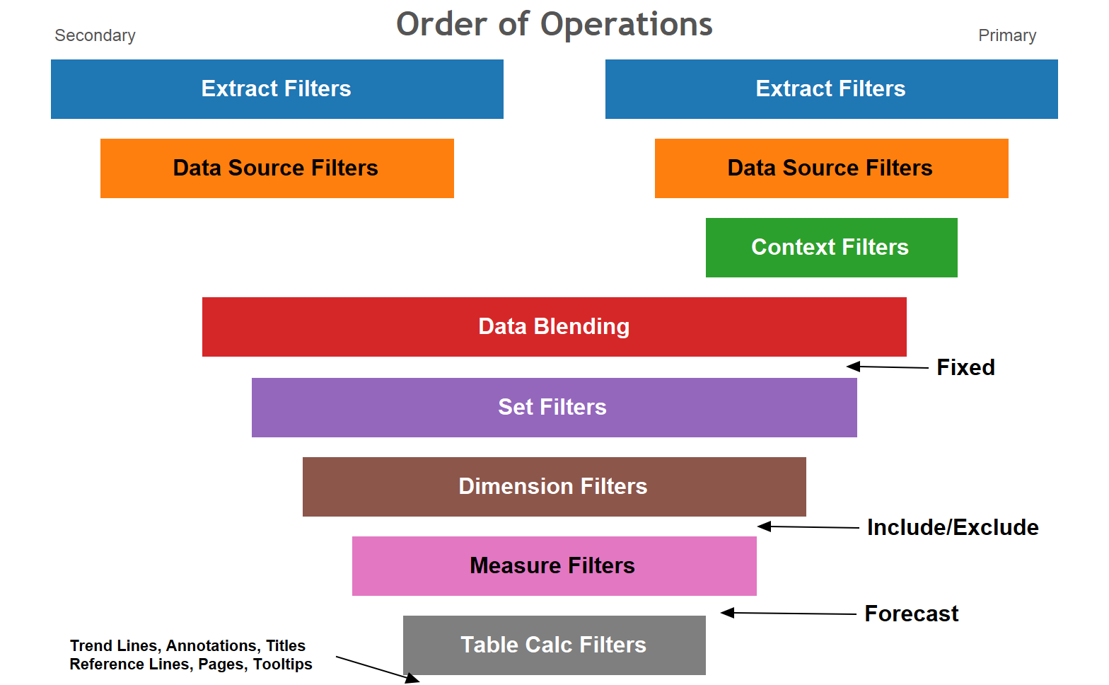
Tableau Conference 2015 this month in Las Vegas, Jen Vasser, a sales consultant at Tableau presented her version of the order of operations or the Query Pipeline. She included:

• Data Blending 
• Forecast
• Annotations, Reference Lines, Trend Lines, Tooltips, Pages, Titles

Last month (September 2015), I updated the diagram to include Set Filters and called it the Precedence of Filtering. Note that I make the pipeline get narrower when going down, because all but the last filters are reducing the data set at the record level. The data set is getting smaller and smaller.

The context filters are actually regular filters that we have manually assigned higher priority in execution. On the other hand, all filters provide context for the filters that follow.

Changing / Swapping Data-source for Duplicated Worksheet

    How to set up  worksheets which I can re-use with different filtered data /data source ?

1. Copy the Tableau file (or save as different name). Now you have FileA and FileB.
2. Open up FileB and replace data source with your new datasource. 
3. When that is done, open up FileA and Copy/Paste the workbooks/dashboards you want from FileB to FileA. 
4. These should now have the new datasource and FileA still has the original datasource. Keep going for as many datasources as you have.

Advance PARAMETER in Tableau

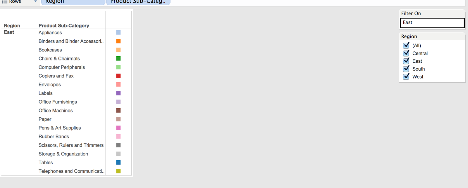
The following example shows how to create a single text box on a dashboard that filters a list of customers by Region or Product Sub Category. To create this type of filter, you will need to create a parameter, a calculated field, and a filter.

Note: Use this strategy when you want to filter on a single value at a time. For example, looking at only the East or only Tables products.

Create the parameter

The first thing you will need to create is a parameter. The parameter is where users will type in the Region or Product Category values.

Step 1 

Connect to your data source. This example uses the Sample - Superstore data source.

Step 2 

Right-click an empty area in the Data window and select Create Parameter.

Step 3 

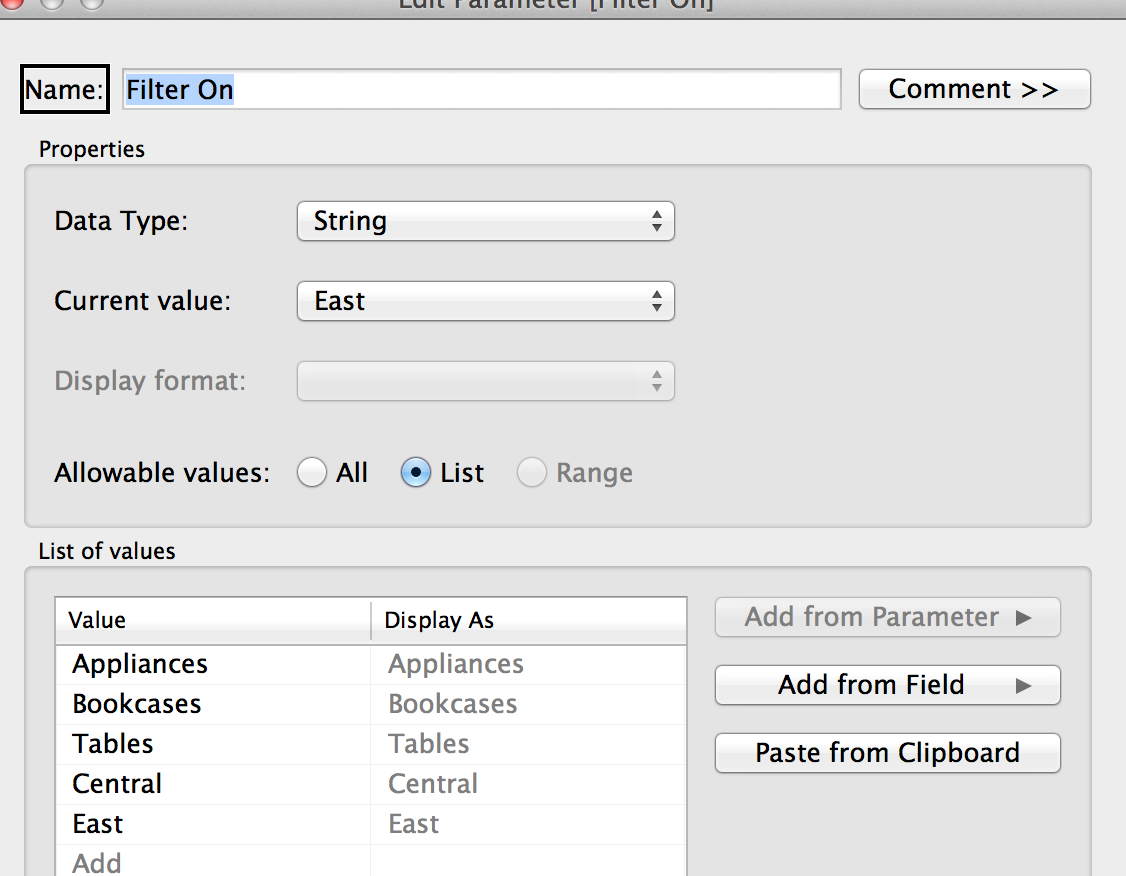
In the Create Parameter dialog box, give the parameter a name such as Filter On. Then specify the parameter settings.

Step 4

Create a calculated field

Now that you have a parameter to collect the value you want to filter on, you need some way of specifying the filter. You can do that by writing a calculated field that compares the Region and Department values to the Filter On value.

Sub Step 1 

Select Analysis > Create Calculated Field.

Sub Step 2 

In the Calculated Field dialog box, do the following tasks:

1. In the Name text box, type Show in View.
2. In Formula text box, type the formula below, and then click OK.

if [Region]=[Filter On] and [Product Sub-Category]!=[Filter On] then 'Select'

ELSEIF [Region]!=[Filter On] and [Product Sub-Category]=[Filter On] then 'Select'

else 'Ignore' END

Step 5

Filter the view

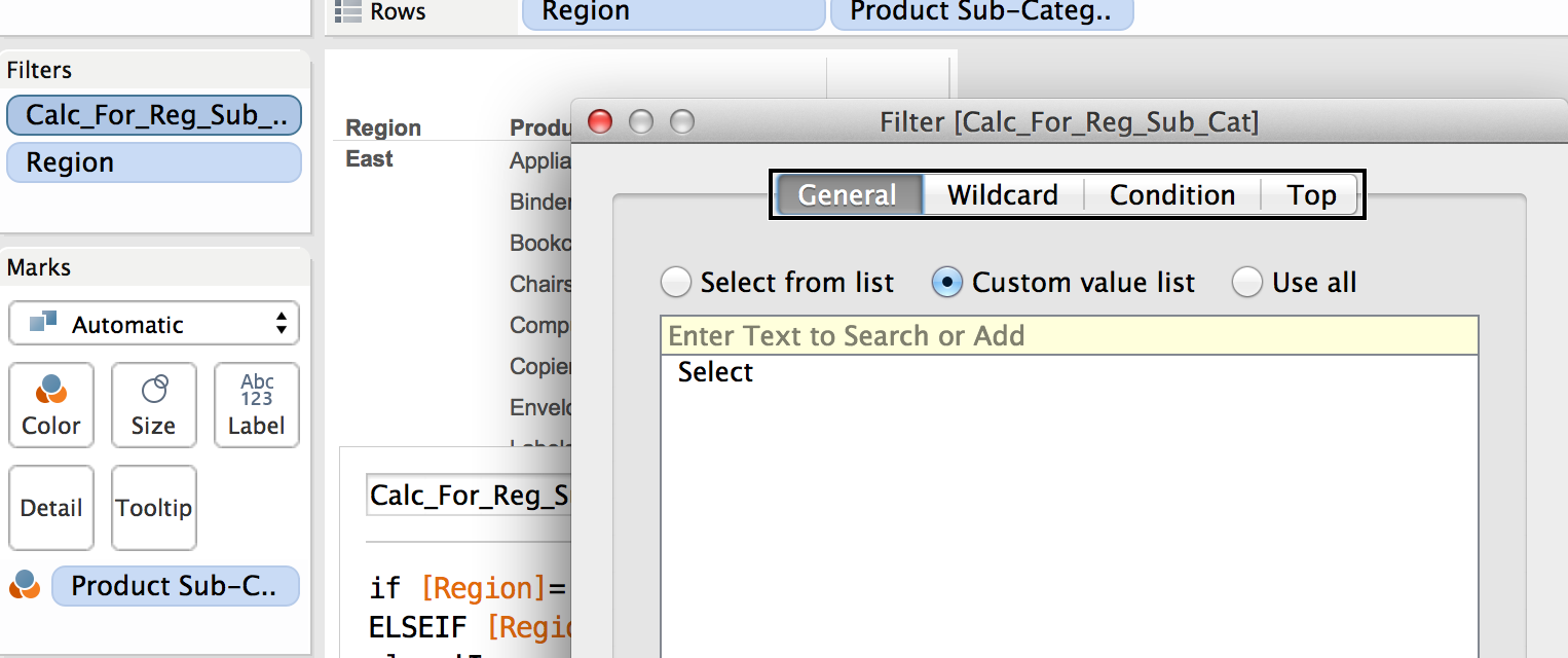
The final step is filtering the view to only include the rows that were marked as "Select." (Note you have to first enter select then click on '+' button)

Step 6

When finished, click OK.Build the view

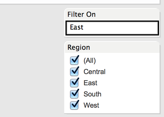
Now that you have all the pieces, build the view you want. Make sure you show the parameter control by right-clicking the parameter in the Data window and selecting Show Parameter Control.

Addressing and Partitioning

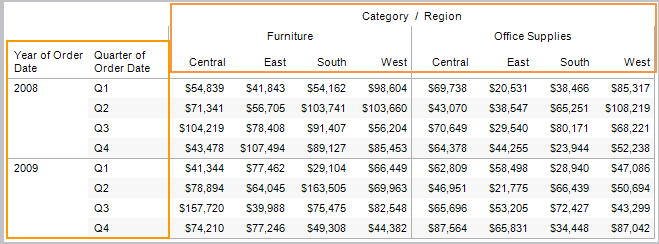
Table calculations are performed on a single measure in the view. The dimensions that define the part of the table you are applying the calculation to (computing along) are called addressing fields, and the dimensions that define how to group the calculation are called partitioning fields. In the example of a running sum of product sales across several years, the addressing field is the Date field, and the partitioning field is the product field. When you define the addressing for a table calculation, all the other dimensions are used for partitioning.

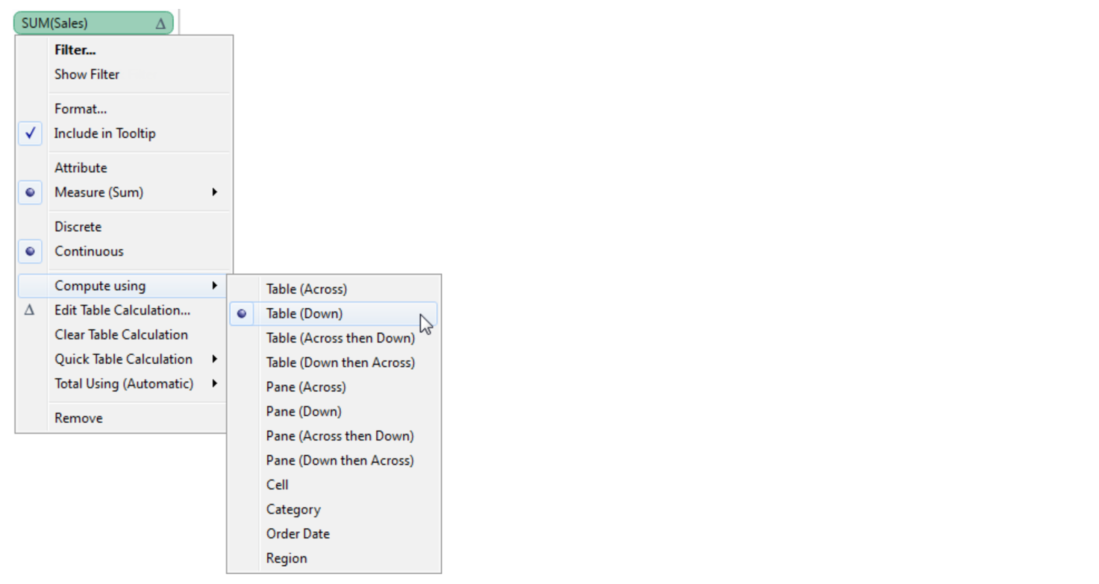
You specify addressing when you create or edit a table calculation, in the Table Calculation dialog box. To update addressing for a field in the view that already has a table calculation, right-click the field and choosing one of the options under Compute using. For example:

Addressing can be relative to the table structure (options beginning with Table, Pane, or Cell) or to a specific field (such as Category, Order Date, or Region). Addressing options based on table structure are described below.

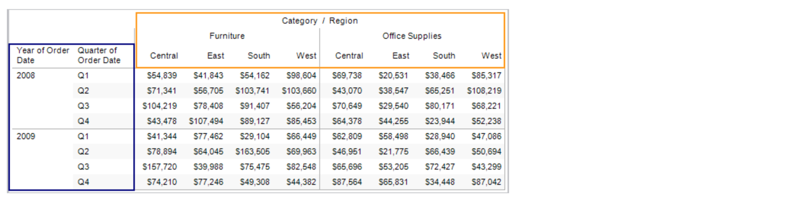
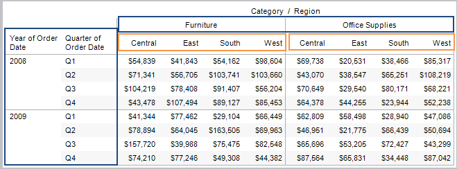
Table (Across)

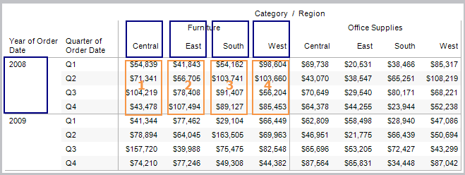
This option sets the addressing to compute along the entire table moving horizontally through each partition. For example, the view below shows quarterly sales by region and product category. When a calculation addressing is set to Table (Across), the dimensions that span horizontally across the table are the addressing fields (in the view below, Category and Region). All the other dimensions (Year, Quarter) are partitioning. The addressing dimensions are shown in orange, while partitioning dimensions are shown in blue.

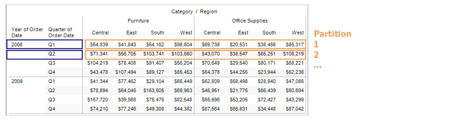
That means that each partition will be the combination of Year and Quarter. Any calculation that is performed is scoped to the partition. For example, if the calculation is percent of total, the calculation will be performed on the numbers within each of the orange boxes.

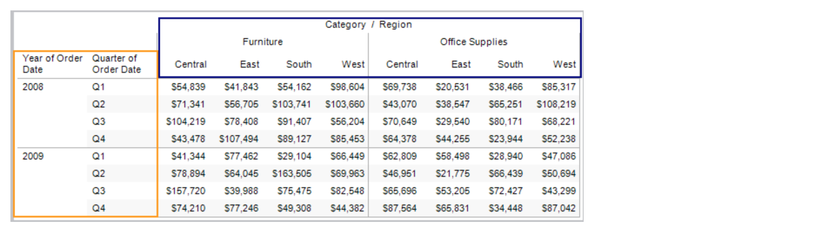
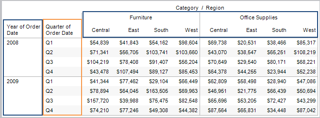
Table (Down)

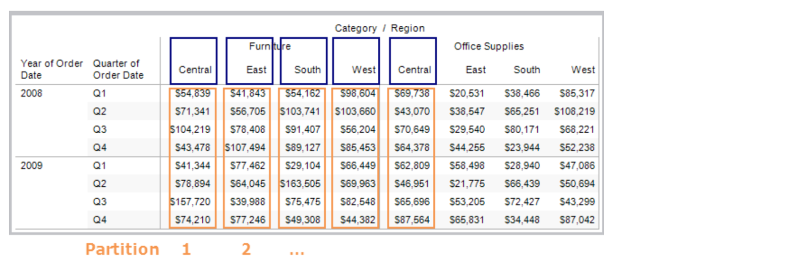
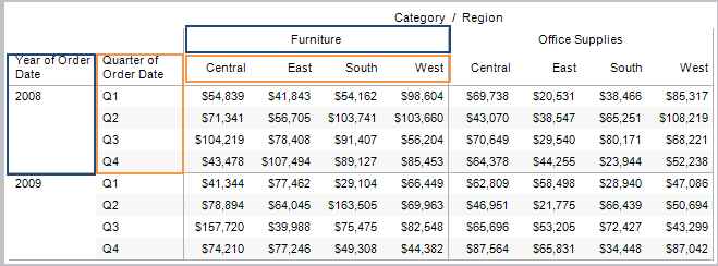
This option sets the addressing to compute along the entire table moving vertically through each partition. For example, the view from above is shown below with the addressing set to compute along Table (Down). The fields that span vertically (Year, Quarter) are now the addressing fields and the rest of the fields are partitioning (Category, Region). The addressing fields are shown in orange while partitioning fields are shown in blue.

That means that each partition is the combination of Category and Region.

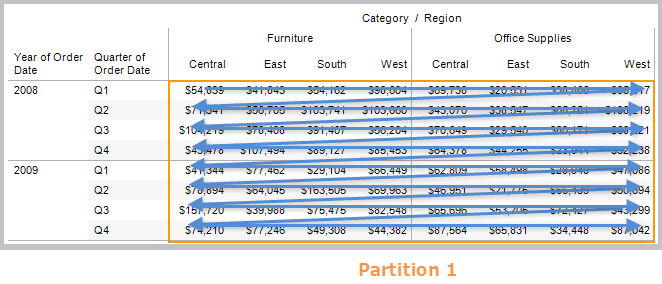
Table (Across then Down)

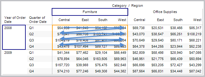
This option sets the addressing to compute across the entire table horizontally and then down the table vertically. This means that both the fields that span across the table and down the table are addressing fields.

That means that the entire table is the partition. The computation will compute across, move to the next row and continue to compute across, and so on.

Pane (Across)

This option sets to compute across the pane horizontally. The fields that span across the pane horizontally are the addressing fields. However, the fields that separate the panes are now partitioning fields. In the example below Category becomes a partitioning field along with Year and Quarter. Region is the addressing field.

That means that the combination of Year, Quarter, and Category is the partition.

Pane (Down)

This option sets the addressing to compute down the table within the pane. The fields that separate the pane (Category, Year) are partitioning fields. In addition, Region becomes a partitioning field and Quarter is the addressing field.

That means that the combination of Year, Category, and Region is the partition.

Pane (Across then Down)

This option sets the addressing to compute across within the pane, then move to the next row and continue to compute across. The addressing fields are both the fields that run across the table horizontally and down the table vertically (Region, Quarter). The partitioning fields are the fields that define the pane (Category, Year).

That means that the combination of Category and Year make up the partition.

Cell

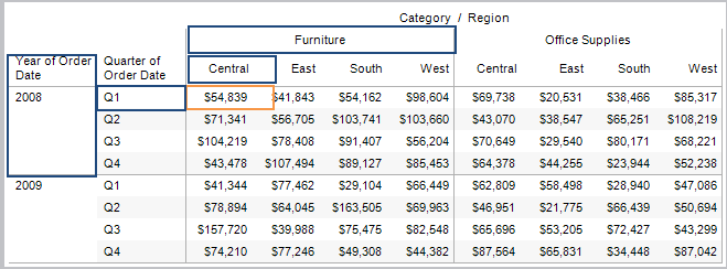
This option sets the addressing to the individual cells in the table. All fields become partitioning fields. This option is generally most useful when computing a percent of total calculation.

That means that the partition is the combination of Category, Region, Year, and Quarter.

Individual Fields

The individual dimensions in the view are listed below the option above in the Table Calculation dialog box. Use them to set the addressing to compute using the field you specify. The benefit of this option is that you get absolute control over how the calculation will be computed—if you change the orientation of your view, the table calculation will continue using the same fields for addressing and partitioning. Be careful though, because, addressing on an individual field means that when you rearrange the table, the calculation may no longer match the table structure.

Advanced

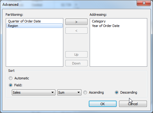
The advanced option lets you specify multiple fields to act as the addressing fields. When you select Advanced, a dialog box opens where you can specify one or more fields to act as addressing fields. Then you can specify how to order those fields.

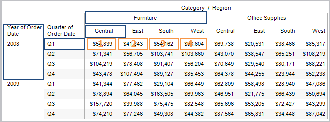
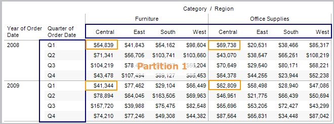
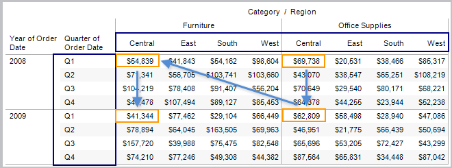
For example, in the view below the addressing fields are set to Category and Year. These are ordered by SUM(Sales), in descending order (from greatest to least). That means that the combination of Quarter and Region create the partition. Q1 Central exists four times in the table, and that is the partition.

Because the order is set to SUM(Sales), the calculation is computed based on their SUM(Sales) values from highest to lowest.

Adding Data Refresh Time Stamp to a View in a Dashboard

Published: 25 Jan 2013

Last Modified Date: 09 Sep 2014

Question

How to add a time of the last data refresh (a time stamp) to a view in a dashboard.

Environment

Tableau Desktop

Answer

Option 1: Add the time stamp to the top of the view

1. Open the workbook that contains the dashboard in Tableau Desktop, and then navigate to the sheet for which you want to display the time of the last data refresh.
2. Select Worksheet > Show Title.
3. Double-click the title.
4. In the Edit Title dialog box, select Insert > Data Update Time, and then click OK.

Option 2: Add the time stamp to the bottom of the view

1. Open the workbook that contains the dashboard in Tableau Desktop, and then navigate to the sheet for which you want to display the time of the last data refresh.
2. Select Worksheet > Show Caption.
3. Double-click the caption.
4. In the Edit Caption dialog box, select Insert > Data Update Time, and then click OK.

Additional Information

The Data Update Time value depends on the type of connection:

• Extract-based connections display the last time the extract was refreshed.
• Live database connections display the last time the data source was refreshed.
• Live file-based connections display the last time the file was updated.