Concept of Box Plot (Tableau)

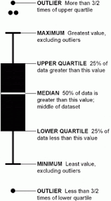
Box -plot is one of the prominent feature important for TABLEAU Statistics section of Examination. Below is simple example to clarify the concept for the individuals new to it.

A small example should make things clear. Consider a small village with 25 inhabitants. This is what they earn and the resulting box plot:

Citizen Nr.	Income	Key Value
25	3,001.25	Maximum
24	2,996.45
23	2,919.35
22	2,787.02
21	2,784.72
20	2,696.83
19	2,412.51	Q3: 0.75 * 25 = 18.75 = 19.
18	2,400.43
17	2,367.84
16	2,333.37
15	2,285.53
14	2,214.87
13	2,069.79	Median: 0.5 * 25 = 12.5 = 13.
12	1,923.62
11	1,819.22
10	1,773.34
9	1,597.54
8	1,589.48
7	1,494.65	Q1: 0.25 * 25 = 6.25 = 7.
6	1,423.74
5	1,391.92
4	1,334.88
3	1,184.53
2	1,125.78
1	1,005.85	Minimum

As you can see, the basic idea is to sort the data and then select the minimum, the maximum and the values at the referring positions: median (0.5), lower (Q1) (0.25) and upper quartile (Q3) (0.75). Why these values are considered to be robust statistic key values? In order to explain this, consider a similar village with one rich person and the following incomes:

Citizen Nr.	Income	Key Value
24	10,345.67	Maximum
23	2,919.35	Upper Bound
22	2,787.02
21	2,784.72
20	2,696.83
19	2,412.51
18	2,400.43	Q3: (18. + 19.)/2 = 2,406.47
17	2,367.84
16	2,333.37
15	2,285.53
14	2,214.87
13	2,069.79
12	1,923.62	Median: (12. + 13.) / 2 = 1,996.71
11	1,819.22
10	1,773.34
9	1,597.54
8	1,589.48
7	1,494.65
6	1,423.74	Q1: (6. + 7.) / 2 = 1,459.2
5	1,391.92
4	1,334.88
3	1,184.53
2	1,125.78
1	1,005.85	Minimum / Lower Bound